How Well do Land Classification Algorithms Detect Community Structure Patterns in Forest Ecosystems?

Last fall I had a meeting with Jean Burns and her former undergraduate student, India Johnson, about using remote sensing to study invasive species.  Among various options, we discussed using artificial intelligence methods to identify and demarcate abundance and distribution patterns of invasive species.  I had already had some experience with semi-automatic classification of land cover using the SCP Plug-in module for QGIS (Congedo, Luca, (2021). Semi-Automatic Classification Plugin: A Python tool for the download and processing of remote sensing images in QGIS. Journal of Open Source Software, 6(64), 3172, https://doi.org/10.21105/joss.03172), and I hadn't had much success with identifying patterns of distribution of the dominant tree species in the north woodlot of CWRU's University Farms.  With this post, I will provide an initial assessment of the limitations of land classification methods when applied to forested ecosystems.

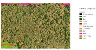
For this assessment, I am using two different sources of multispectral imagery (Figs. 1 and 2).  Most of the UAV images are from a Sentera Double 4K Multispectral Sensor with  RGB (narrow band red, green, and blue bands) and NIR (red edge and near infrared bands) cameras. At 150 m, these images have a pixel resolution of 3 cm and the raster has about 240 million pixels.  I have recently discovered the availability of high resolution, multispectral images from Planet (Planet Application Program Interface: In Space for Life on Earth. San Francisco, CA. https://api.planet.com).  The image in Fig. 2 contains about 500,000 pixels with a resolution of 3m.  There are obvious patterns of land cover in both images, and there appear to be discernible patterns of distribution of different tree species in the high resolution image of the north woodlot (Fig. 1). 

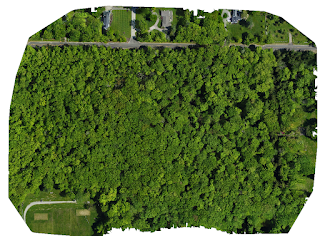
Figure 1.  Ortho-mosaic image of the north woodlot of University Farms on May 26, 2020 based on 136 individual images from the RGB camera of the Sentera Double 4K Multispectral Sensor with a pixel size of 3.1 cm.

 

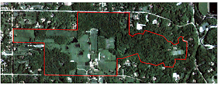
Figure 2.  Satellite image of the University Farm property (outlined in red).  Satellite image is a PSScene4Band image from Planet on June 8, 2020, with a pixel size of 3 m.

The SCP module in QGIS has two methods of generating land cover classifications.  Supervised classifications require an a priori training input to establish spectral signatures of land cover categories.  In contrast, unsupervised classifications builds a land cover classification by clustering pixels by similarity of spectral signatures.  Fig. 3 is an example of a supervised classification of the north woodlot.  Although the patterns are similar, the classification produces a different distribution of forest features.  The main obstacle to improving the classification is substantial overlap of spectral signatures of the various tree species used in the training input.  

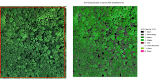
Figure 3.  Comparison of part of the north woodlot in Fig. 1 (left panel) with the results of a supervised classification of the forest canopy of the north woodlot using the SCP module in QGIS (right panel).  The classification required manual specification of regions of interest for each of the categories.  

Fig. 4 provides an example of unsupervised classification of the image in Figure 1.  A challenge with is identifying land cover categories associated with clusters arising from the unsupervised classification.  Areas of grass cover or roads and other built features are easy to identify, but the structure of the forest canopy is much harder to classify by species.  Gaps in the forest canopy, however, are well demarcated.  High resolution of the image, in fact, leads to detection of gaps in the upper canopy of individual trees.  

Figure 4.  Results of supervised classification of forest features from image in Fig. 1.

The 3 m pixel resolution of the Planet satellite imagers provides a lower resolution option for exploring forest structure.  The feature categories in Fig. 5 lack correspondence with features in Fig. 4, except for gap areas.  The lower resolution satellite images result in identification of the larger areas between individual tree canopies.  The also reveal areas of similar spectral signatures that may not be species specific.

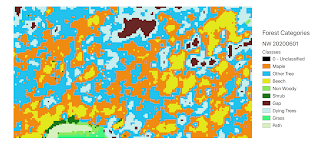
Figure 5.  Results of unsupervised classification of forest features in the north woodlot from PSScene4Band image in Fig. 2.

The reason for the lack of species specific spectral signatures in either Fig. 4 or Fig. 5 likely involves variation in the observable structure of tree canopies.  Fig 6, is a high resolution image of 76 x 57 m area within the north woodlot.  At this scale of resolution, it is possible to identify maple and oak leaves.  Although there is a slight difference in the perceived color of maple and oak branches, the coloration is not constant at different heights in the overall canopy.  Thus spectral signatures of lower leaves in the canopy will be different from upper leaves.  Also, the gaps between branches  is not species specific.  Both supervised and unsupervised classifications are limited by the overlap of spectral signatures associated with the physical structure of individual tree canopies.   

  

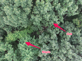
Figure 6. UAV image taken on July 24, 2017, in the north woodlot.  The image was acquired with a Phantom drone at 60 m altitude.  Individual pixel size is 1.9 cm and the width of the image is 76 m.  Arrows indicate maple and oak tree canopies.

Conclusion

Although individual leaves of tree species in the north woodlot are easy to distinguish by size, shape, and color, demarcation of individual tree species with remote sensing methods seems impractical.  The substantial overlap of spectral signatures of different species leads to unreliable categorization.  Because much of the overlap arises from the physical structure of the canopy, however, some categories will be more consistently identified.  For example, gap structure of the canopy varies with resolution of images, but is largely consistent (compare Figs. 4 and 5 for location of major canopy gaps).  Uppermost leaves of some tree species likely have  distinctive  spectral signatures.  Determining whether those are sufficiently distinctive of account for the other patterns in Figs 4 and 5 remains a work in progress.

Are Long-term Data Sets Worth the Effort at Biology Field Stations?

For the past 11 years, I have been maintaining equipment and curating data sets for environmental monitoring at University Farms of Case Western Reserve University.  Although the original deployment of was part of my research on Great Lakes ecosystems, the environmental monitoring program at the CWRU Farm became a general resource for research and education.  The original monitoring began with two weather stations, one in an open field and the other in the north woodlot.  Later, we added hydrology monitoring of the experimental watershed and additional environmental monitoring associated with the Farm’s Food Production Program.  The former Farm Director, Dr. Ana Locci, supported and encouraged this work as part of an effort to improve the research and education infrastructure at the Farm.  Our partnership on environmental monitoring platforms deepened with the arrival of Beech Leaf Disease (BLD) at the Farm in 2017 and led to incorporation of a remote sensing platform with the addition of an unmanned aerial vehicle and sensors to monitor changes in forest canopies associated with the spread of BLD.  I summarized preliminary findings of this work in previous posts.  In this post, I want to reflect on the value of long-term monitoring at a university field station.

The motivation for this reflection has arisen from both personal and institutional changes in priorities.  As with many things over the last two years, the Covid-19 pandemic has contributed to reassessment of research and education initiatives at the Farm.  With Dr. Locci’s retirement as Farm Director in 2020, the environmental monitoring program lost its primary institutional sponsor.  In the hiatus following her retirement, restrictions on activities associated with the University’s Covid protocols, led to shorter-term reassessment of priorities of Farm management and activities of the Biology faculty involved with the Biology Field Station.  Along with these changes and changes in my personal priorities, the environmental monitoring program has now ended.  Only the weather station in the north woodlot and a weather station at the November Greenhouse continue operating, and this will be the last year for which the remote data logger in the north woodlot will report data over a 3G network.  Recently, however, some CWRU faculty have asked for access to historical environmental data.  In particular, Dr. Mark Green and his undergraduate student, Kyle Rickert, have analyzed some of the weather station data as part of a small project to measure sap flux in beech trees of the north woodlot.  Although I had proposed providing a data archiving platform for Farm data in 2018, I haven’t kept up with documenting a wide range of problems with the monitoring platforms.  Various probe failures, data gaps, and difficulties accessing historical data made it difficult to give others access to a consistent set of time series from various probes.  Stimulated by Green and Rickert’s preliminary analyses of partial data sets, I have now finished a complete review of the data and am distributing the consolidated data from the weather station to interested researchers.  As of January 20, 2023, the data from the Farm weather stations is now publicly available (see References below).

In their partial analysis of soil moisture data from the north woodlot weather station, Green and Rickert found some recent increases in the soil moisture that reinforced their observations of reduced sap flux in BLD infected beech trees.  Previously, Dr. Locci and I had identified a pattern of increased solar radiation in the north woodlot where damage to beech was acute.  To me, the following Figures 1 and 2, prove the importance of maintaining long-term environmental monitoring at the Farm.  

In my first post on BLD incidence at the Farm (2017 post), I noted that the ratio of solar radiation measured at the weather stations of the north woodlot and open field had nearly doubled from a about 6% prior to 2017 to about 12% in 2017 during the summer.  As illustrated in Fig. 1, this trend continued after 2017 with the ratio approaching 19% in the summer of 2021.  Fig. 2 also shows a substantial change in soil moisture from 2017 to 2021.  Over the period of 2009 to 2016, minimum fall soil moisture (m3/ m3) ranged from 0.02 to 0.1, except for 2014.  From 2017 to 2021, minimum soil moisture increased to 0.1 in 2017 and 2018 and then to 0.22 in 2021.  

Conclusion

The eastern part of the north woodlot is a remnant primary forest with a predominant beech-maple assemblage. Beech Leaf Disease is only the latest stressor on beech in northeastern Ohio.  Beech bark disease has also impacted the beech area of the north woodlot.  The cumulative stress on beech trees is evident is the loss of large old beeches.  Without the long-term data sets from the weather stations, however, it would have been difficult to detect the timing of the consequences of these stressors.  The increases in the fall soil moisture from 2017 correspond most closely with the outbreak of Beech Leaf Disease.  It would thus seem prudent to continue this environmental monitoring program.

References

Koonce, J.F. 2023. Weather data for the period 2016 to 2022 from the HH1 Greenhouse location at University Farms, Case Western Reserve University ver 1. Environmental Data Initiative. https://doi.org/10.6073/pasta/33776fc6b8588fecc802db8405cfad3f (Accessed 2023-01-18).

Koonce, J.F. 2023. Weather data for the period 2009 to 2022 from the North Woodlot location at University Farms, Case Western Reserve University ver 4. Environmental Data Initiative. https://doi.org/10.6073/pasta/abe2eb0ba198d3faf682e0245b5eedaa (Accessed 2023-01-20).

Koonce, J.F. 2023. Weather data for the period 2009 to 2022 from the Open Field location at University Farms, Case Western Reserve University ver 3. Environmental Data Initiative. https://doi.org/10.6073/pasta/67e5f60b87c38157f5240a5546ece0af (Accessed 2023-01-20).

Changes in Upper Canopy of Farm North Woodlot in 2019

The previous post summarized the lack of evidence that Beech Leaf Disease was having an effect on the upper canopy of a woodlot at CWRU’s University Farms in Hunting Valley, Ohio.   Continuing observations in the spring and early summer of 2019, however, suggest that the forest canopy is changing.  During the winter of 2018/2019, several large beech trees in the Farm’s north woodlot fell out of the canopy.  These oldest beeches had survived a number of pathological stresses and continued the pattern of gradual losses of the oldest beech trees.  The purpose of this post is to document the changes in the forest canopy of the north woodlot observed during drone surveys in the spring and early summer of 2019.

Drone surveys of the north woodlot during 2019 concentrated on imagery from a multispectral sensor.  The Sentera Double 4K Multispectral Sensor has two cameras, the RGB camera captures reflectance in three narrow visible light bands of red, blue, and green and the the NIR camera captures red edge and near infrared bands.  Figure 1 shows the spectral characteristics and quantum efficiency of the sensors.

Figure 1.  Manufacture’s spectral specifications for the Sentera Double 4K Multispectral Sensor, showing the quantum efficiency of the five spectral bands captured by the sensor’s two cameras.

The images from the sensor cameras capture light reflectance from the landscape.  Plants absorb and reflect light in the visible spectrum and reflect light at wavelengths greater than 700 nm (Gates et al. 1965, Gao et al. 2000).  For this work, I have chosen to use the normalized difference red edge index (NDRE):

NDRE = (NIR – RE)/(NIR + RE)

Figure 2 is an NIR orthoimage of the north woodlot on July 19, 2019 that I created with OpenDroneMap, which is an open source drone mapping software application.  Figure 2 is a composite image of the red edge and near infrared bands from the Sentera Double 4K NIR camera.  Using the raster calculator in QGIS, I created the NDRE orthoimage in Figure 3 from the red edge and near infrared bands in Figure 2.  Because the quantum efficiency of red edge is greater than near infrared, the NDRE index has negative values.

Figure 2.  OpenDroneMap orthomosaic of images taken on July 19, 2019 with the Sentera Double 4K Multispectal Sensor’s NIR camera, which captures Red Edge and NIR reflectance spectra.  Red dots represent the locations of recent tree falls, which created openings in the canopy.

Figure 3.  NDRE index raster calculated from the red edge and near infrared bands in Figure 2.  White areas correspond to high values of the NDRE index and darker areas to lower values of the index.  Red dots indicate position of large tree falls.

Figure 4.  Raster histogram of the NDRE index raster in Figure 3. 

Although the composite image from RGB camera of the Sentera sensor is not true color, the orthomosaic from the RGB images provides a composite visible color reflectance of the north woodlot (Figure 5).  The red dots in Figure 5 show locations where large tree falls occurred and the canopy gaps appeared.  These same areas appear as “white” areas in the NDRE index raster (Figure 3).

Figure 5.  Composite orthomosaic of the north woodlot from RGB camera images on July 19, 2019.  The orthomosaic location corresponds to the location of the orthomosaic in Figure 2.

The pattern of variability of the NDRE index in Figure 3 is quite different from the patterns observed in 2018.  Figure 6 shows the NDRE index pattern observed in June 2018, and Figure 7 shows the pattern observed in August 2018.  The raster histograms are also different with those from both 2018 dates showing markedly less skew toward higher values (Figure 8).

Figure 6.  NDRE index raster calculated from the red edge and near infrared bands of the NIR orthomosaic from sensor images taken on June 19, 2018.

Figure 7.  NDRE index raster calculated from the red edge and near infrared bands of the NIR orthomosaic from sensor images taken on August 10, 2018.

Figure 7.  NDRE index raster calculated from the red edge and near infrared bands of the NIR orthomosaic from sensor images taken on August 10, 2018.

Preliminary Conclusions

In contrast to observations in 2018, it appears that the north woodlot upper canopy is beginning to show substantial changes in NDRE index values in 2019.  Apart from gap openings associated with the loss of large beech, the increase in the “light” colored areas is an indication of widespread deterioration in the apparent health of the canopy in the beech dominated areas of the north woodlot.  Future posts will provide more detailed analysis.

References
Gates, D. M., H. J. Keegan, J. C. Schleter, and V. R. Weidner.  1965.  Spectral Properties of Plants.  Applied Optics, 4(1):11-20.

Gao, X., A. R. Huete, W. Ni, and T. Miura.  2000.  Optical-Biophysical Relatonships of Vegetation Spectra without Background Contamination.  Remote Sens. Environ. 74:609-620.

Effects of Beech Leaf Disease on Upper Canopy in 2018

Following the previous post about Beech Leaf Disease, I have continued collection of environmental data and begun acquisition of imagery from UAV drones to explore the continuing effects of BLD on the forest in the north woodlot of University Farm.  The purpose of this post is to report preliminary observations about the lack of a discernable effect of BLD on the upper canopy of the forest and to update observations of BLD incidence in 2018.

The BLD incidence in University Farm’s north woodlot in 2018 was similar to observations in 2017.  Figure 1 illustrates the same diminished leaf growth in the secondary canopy of the north woodlot observed in 2017.  Figure 2 is a close up view of the effect of BLD on beech leaves, showing the characteristic darkening of the area between leaf veins.  Later the number of leaves showing the effects of BLD will increase and the leaves eventually shrivel and drop off.

Figure 1.  Openness of the secondary canopy in late June 2018 in a beech dominated area of the north woodlot of Case Western Reserve University’s University Farm.  The photo is north facing in the vicinity of the north woodlot weather station.

Figure 2.  Close up view of infected beech leaves in the secondary canopy of the north woodlot of University Farm.

As in 2017, the light levels in the beech dominated area of the north woodlot increased relative to the levels prior to 2017.  The ratio of forest incident solar radiation to open field solar radiation remained about double the levels in June to September of 2015 and 2016 (Figure 3). 

Figure 3.  Ratio of forest to open field incident daily-averaged solar radiation observed at weather stations in University Farm.  

I monitored upper canopy foliage changes with two drone platforms.   The DJI Phantom 3 Standard drone used in 2017 had a 12 megapixel camera with Red, Green, and Blue color bands.  The DJI Inspire 2 drone used in 2018 carried either a 20 megapixel,  Zenmuse X4s camera or a Sentera Double 4K Multispectral sensor.  Both the Phantom 3 camera and the Zenmuse X4s take true color images using red, green, and blue color bands.  The Sentera sensor has two cameras.  One camera captures narrow red, green, and blue color bands, and the other has red edge and a near infrared color bands.  University Farms’ Facebook page has links to two short videos (Link 1 and Link 2) about the use of the Inspire drone and its cameras.  This post summarizes some of initial findings from examination of individual images.  Future posts will more fully document collection, processing, and analysis of the imagery.

Drone mounted cameras and sensors provide detailed views of the canopy structure and leaf condition in the north woodlot.  I first focus on the imagery of the upper canopy near the north woodlot weather station where the effects of BLD on the secondary canopy are most clear (see Figure 1).  Figures 4 and 5 show a portion of the north woodlot with an area of leaf damage in the upper canopy of a beech tree (highlighted by a red outline).  Damage in 2017 (Figure 4) seems less severe 15 months later (Figure 5).  Figure 6 and 7 are enlarged views of the red outline areas in Figures 4 and 5.  In Figure 6, the leaves appear sparse, under developed, and yellowed.  BLD infected leaves in the secondary canopy, in contrast are thickened and darker than uninfected leaves.  It thus seems unlikely that this type of damage is the result of BLD.

Figure 4.  Copy of a jpeg image from the DJI Phantom 3 Standard color camera on July 24, 2017 in the vicinity of the north woodlot weather station.  The photo was taken at 45 m altitude.  The area outline in red shows evidence of leaf damage in the upper canopy.

Figure 5.  Photo taken on September 17, 2018 at the same location as in Figure 4, in the vicinity of the north woodlot weather station.  Image taken with a DJI Phantom 3 standard camera at an altitude of 45 m.  Area highlighted with a red outline is the same as the area outline in Figure 4.

Figure 6.  Closer look at canopy damage in the red outline area of Figure 4 from July 24, 2017.  Damage is to part of the canopy of a beech tree showing diminished leaf grow.  The affected leaves do not seem to show the characteristic thickening of BLD infected leaves.

Figure 7.  Close up of red outlined area in Figure 5 taken on September 14, 2018.  The close up is directly comparable to the image in Figure 6 and shows general recovery and possible loss of canopy structure a year after the damage viewed in Figure 5.

Although the drone imagery reveals some areas of upper canopy damage, determining the cause of the damage is difficult.  Beech in the eastern portion of the north woodlot have been under stress for many years.  The eastern part of the north woodlot is a remnant primary forest.  More than 50 years ago, beech dominated this area, and finding beech trees with diameters (DBH) of more than 100 cm was common.  Nearly all of those large beech have fallen out of the canopy.  As in Figure 4, there are also many standing dead beech trees, and all of this mortality occurred before BLD appeared. 

Because the drone imagery provides an overview of the entire north woodlot, it is possible to check more systematically for patterns of upper canopy damage.  A wide variety of vegetation indices have proven useful in vegetation surveys for agriculture and forestry, and I began to explore using some of these indices to identify potential BLD effects.  I next focus on the results from the TGI and NDRE vegetation indices.  I chose these two indices because they use light bands from each of the two cameras on the Sentera Double 4K Multispectral Sensor that I mount on the DJI Inspire 2 drone.  The spectral bands are, Blue (446nm x 60nm width),  Green (548nm x 45nm width), Red (650nm x 70nm width),  Red Edge (720nm x 40nm width) and Near Infrared (840nm x 20nm width).  The two vegetation indices (calculated for each pixel in the image are as follows:

            TGI = Green - 0.39*Red -0.61*Blue

            NDRE = (NIR – RE)/(NIR + RE)

Using an R script with the rgdal and gdalUtils libraries, I transformed each drone image into a GeoTiff raster for each vegetation index and sampled the mean value of the vegetation index from the raster values within a 1.5 m radius circle centered on a sample point in a set of specified sample locations.  Creating a regularly distributed set of 200 sample points for the north woodlot provided a standard way to analyze both spatial and temporal variability of the indices.  Figure 8 shows that the two indices are inversely correlated with a highly significant correlation coefficient of 0.64 and an RSQ value of 0.406.

Figure 8.  Scatter plot of the association of the mean NDRE and mean TGI vegetation indices for two hundred sample locations in the north woodlot.  The correlation had an RSQ value of 0.41 and was significant at the 0.001 level.  Also shown is the regression in blue and standard error band in grey.

To facilitate comparisons of forest areas with and without beech, I created a set of spatial polygons.  Three of the polygons were located in forest areas dominated by beech, including one area used by researchers from Holden Arboretum to study effects of adding fertilizer to forest plots.  The other two areas were in oak and maple dominated areas.  Each of the spatial polygons included a minimum of 4 of the 200 standard sampling points used for all pattern analysis.  Figures 9 and 10 provide summaries of temporal variability of TGI and NDRE indices.  I want to emphasize two aspects of the results.  First, neither vegetation index shows consistent differences in order or values of the three types of sample areas.  Second, the NDRE vegetation index seems more sensitive to changes in leaf irradiance after canopy closure.  Figure 11 shows that full leaf out and canopy closure was complete by the third week of May when the TGI index reached maximum value.  In contrast, NDRE values did not peak until the second week of June.

Figure 9.  Temporal variability of mean TGI values in three types of areas of the north woodlot at University Farm.  Results are for five spatially defined areas (2 Beech, 1 Beech plot used by Holden Arboretum for fertilizer application, and 2 non-beech).

Figure 10.  Temporal variability of mean NDRE values in three types of areas of the north woodlot at University Farm.  Results are for five spatially defined areas (2 Beech, 1 Beech plot used by Holden Arboretum for fertilizer application, and 2 non-beech).

Figure 11.  Changes in ratio of north woodlot to open field incident solar radiation for the period May 1 to August 31, 2018.

Conclusion

Despite the major effect of BLD on beech trees in the secondary canopy of the north woodlot and the increases in incident solar radiation relative the a 2010 to 2016 baseline, it appears that BLD has had much less effect on the upper canopy.  Existing changes of upper canopy structure (damaged foliage or standing dead trees) seems a continuation of long-duration stress on beech.  Leaf irradiance indices also show little evidence of a specific change in upper canopy beech leaf color or area that we would expect with the changes seen in secondary canopy beech (see Figure 2).